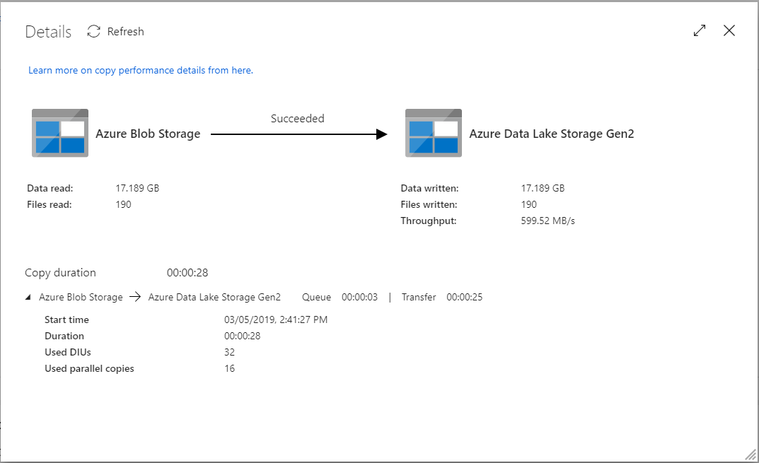
Just created a simple Azure Data Factory job that copies blobs from a container of an Azure Storage account to an Azure Data Lake Store Gen2 account.
Dataset size is 17.2GB/190 files. Copy throughput was 599.52MB/s. Pretty good.
Just created a simple Azure Data Factory job that copies blobs from a container of an Azure Storage account to an Azure Data Lake Store Gen2 account.
Dataset size is 17.2GB/190 files. Copy throughput was 599.52MB/s. Pretty good.
Read it here
This is a very good read: http://www.grahamlea.com/2016/08/distributed-transactions-microservices-icebergs/
You created a SSIS package. The package uses Oracle data sources. Then you can no longer open the package in SSDT/Visual Studio. The error message is “Value does not fall within the expected range” which isn’t quite helpful.
You may need to install the Microsoft Connectors v4.0 for Oracle by Attunity: https://www.microsoft.com/en-us/download/details.aspx?id=52950. After the installation, your SSDT should be able to open the SSIS package again.
Just completed my biggest test query ever on the Presto server I built recently. It joined 1.65 billion rows from 9 tables (sourced from PointClickCare).
Result: 839 million rows (no aggregation done!).
Duration: 1.21 hours.
Cumulative memory: 338PB.
Peak memory: 87.81GB.
The server is an E16S_V3 VM on Azure, which has 16 vCPU and 128GB of RAM. All data read from and written back to Azure Storage Blob in ORC format.
See the screenshots to see how massive the query was!


Sources:
To better understand how partitioning and bucketing works, please take a look at how data is stored in hive. Let’s say you have a table
You insert some data into a partition for 2015-12-02. Hive will then store data in a directory hierarchy, such as:
As such, it is important to be careful when partitioning. As a general rule of thumb, when choosing a field for partitioning, the field should not have a high cardinality – the term ‘cardinality‘ refers to the number of possible values a field can have. For instance, if you have a ‘country’ field, the countries in the world are about 300, so cardinality would be ~300. For a field like ‘timestamp_ms’, which changes every millisecond, cardinality can be billions. The cardinality of the field relates to the number of directories that could be created on the file system. As an example, if you partition by employee_id and you have millions of employees, you may end up having millions of directories in your file system.
Clustering, aka bucketing, on the other hand, will result in a fixed number of files, since you specify the number of buckets. What hive will do is to take the field, calculate a hash and assign a record to that bucket.
FAQ
What happens if you use e.g. 256 buckets and the field you’re bucketing on has a low cardinality (for instance, it’s a US state, so can be only 50 different values?
You’ll have 50 buckets with data, and 206 buckets with no data.
Can partitions dramatically cut the amount of data that is being queried?
In the example table, if you want to query only from a certain date forward, the partitioning by year/month/day is going to dramatically cut the amount of IO.
Can bucketing can speed up joins with other tables that have exactly the same bucketing?
In the above example, if you’re joining two tables on the same employee_id, hive can do the join bucket by bucket (even better if they’re already sorted by employee_id since it’s going to do a mergesort which works in linear time).
So, bucketing works well when the field has high cardinality and data is evenly distributed among buckets. Partitioning works best when the cardinality of the partitioning field is not too high.
Also, you can partition on multiple fields, with an order (year/month/day is a good example), while you can bucket on only one field.
The Hive connector supports querying and manipulating Hive tables and schemas (databases). While some uncommon operations will need to be performed using Hive directly, most operations can be performed using Presto.
Create a new Hive schema named web that will store tables in an S3 bucket named my-bucket:
CREATE SCHEMA hive.web
WITH (location = 's3://my-bucket/')
Create a new Hive table named page_views in the web schema that is stored using the ORC file format, partitioned by date and country, and bucketed by user into 50 buckets (note that Hive requires the partition columns to be the last columns in the table):
CREATE TABLE hive.web.page_views (
  view_time timestamp,
  user_id bigint,
  page_url varchar,
  ds date,
  country varchar
)
WITH (
  format = 'ORC',
  partitioned_by = ARRAY['ds', 'country'],
  bucketed_by = ARRAY['user_id'],
  bucket_count = 50
)
Drop a partition from the page_views table:
DELETE FROM hive.web.page_views
WHERE ds = DATE '2016-08-09'
  AND country = 'US'
Query the page_views table:
SELECT * FROM hive.web.page_views
Create an external Hive table named request_logs that points at existing data in S3:
CREATE TABLE hive.web.request_logs (
  request_time timestamp,
  url varchar,
  ip varchar,
  user_agent varchar
)
WITH (
  format = 'TEXTFILE',
  external_location = 's3://my-bucket/data/logs/'
)
Drop the external table request_logs. This only drops the metadata for the table. The referenced data directory is not deleted:
DROP TABLE hive.web.request_logs
Drop a schema:
DROP SCHEMA hive.web
Using subqueries in where clause for filtering may not work as you expect. Compare the two where conditions:
The two subqueries in #1 return dates ‘2017-12-01’ and ‘2018-01-07’, respectively. So the two should be treated the same, right? Turns out Presto produces completely different plans.
In my test, for #1, presto generated two separate stages for the two subqueries, and pinned them in memory as the “right side” to perform inner joins with the data from other table(s). So table “a” was not filtered using the date range at all, a straight table scan happened, all data was loaded into memory and then “joined” to the two datasets from the sub queries to filter the unwanted rows. Obviously it was a total waste of time and compute resources.
For #2, it was as expected, table “a” was first filtered using the date range, effectively reduced the number of rows loaded into memory, thus the rime & resources required to perform the query was drastically reduced compare to #1.
See the screenshots below to see the difference.


Original post: Protecting Sensitive Information in Docker Container Images
By Matthew Close
Dealing with passwords, private keys, and API tokens in Docker containers can be tricky. Just a few wrong moves, and you’ll accidentally expose private information in the Docker layers that make up a container. In this tutorial, I’ll review the basics of Docker architecture so you can better understand how to mitigate risks. I’ll also present some best practices for protecting your most sensitive data.
It has become fairly common practice to push Docker images to public repositories like hub.docker.com. This is a great convenience for distributing containerized apps and for building out application infrastructure. All you have to do is docker pull your image and run it. However, you need to be careful what you push to hub.docker.com or you can accidentally expose sensitive information.
If you are relatively new to using Docker, they have really great Getting Started Guidesto get you comfortable with some of the topics we will discuss in this tutorial.
To better understand some of the risks associated with using private data in Docker, you first need to understand a few pieces of Docker’s architecture. All Docker containers run from Docker images. So when you docker run -it ubuntu:vivid /bin/bash, you are running the image ubuntu:vivid. Almost all images, even Ubuntu, are composed of intermediate images or layers. When it comes time to run Ubuntu in Docker, the Union File System (UFS) takes care of combining all the layers into the running container. For example, we can step back through the layers that make up the Ubuntu image until we no longer find a parent image.
$ docker inspect --format='{{.Parent}}' ubuntu:vivid
2bd276ed39d5fcfd3d00ce0a190beeea508332f5aec3c6a125cc619a3fdbade6
$ docker inspect --format='{{.Parent}}' 2bd276ed39d5fcfd3d00ce0a190beeea508332f5aec3c6a125cc619a3fdbade6
13c0c663a321cd83a97f4ce1ecbaf17c2ba166527c3b06daaefe30695c5fcb8c
$ docker inspect --format='{{.Parent}}' 13c0c663a321cd83a97f4ce1ecbaf17c2ba166527c3b06daaefe30695c5fcb8c
6e6a100fa147e6db53b684c8516e3e2588b160fd4898b6265545d5d4edb6796d
$ docker inspect --format='{{.Parent}}' 6e6a100fa147e6db53b684c8516e3e2588b160fd4898b6265545d5d4edb6796d

$
The last docker inspect doesn’t return a parent, so this is the base image for Ubuntu. We can look at how this image was created by using docker inspect again to view the command that created the layer. The command below is from the Dockerfile and it ADDs the root file system for Ubuntu.
$ docker inspect --format='{{.ContainerConfig.Cmd}}' 6e6a100fa147e6db53b684c8516e3e2588b160fd4898b6265545d5d4edb6796d
{[/bin/sh -c #(nop) ADD file:49710b44e2ae0edef44de4be4deb8970c9c48ee4cde29391ebcc2a032624f846 in /]}
This brings us to an important point in how Docker works. You see, each intermediate image has an associated command, and those commands come from Dockerfiles. Even containers like Ubuntu start off with a Dockerfile. It’s a simple matter to reconstruct the original Dockerfile. You could use docker inspect to walk up through the images to the root, collecting commands at each step. However, there are tools available that make this a trivial task.
One very compact tool I like is dockerfile-from-image created by CenturyLink Labs. If you don’t want to install any software, you can use ImageLayers to explore images.
Here’s the output of dockerfile-from-image for Ubuntu.
$ dfimage ubuntu:vivid
ADD file:49710b44e2ae0edef44de4be4deb8970c9c48ee4cde29391ebcc2a032624f846 in /
RUN <-- edited to keep this short
CMD ["/bin/bash"]
As you can see, it’s very easy to reconstruct the Dockerfile from an image. Let’s take a look at another Docker image I created. This container has nginx running with an SSL certificate.
$ dfimage insecure-nginx-copy
FROM ubuntu:vivid
MAINTAINER Matthew Close "https://github.com/mclose"
RUN apt-get update && apt-get -y upgrade
RUN apt-get -y install nginx && apt-get clean
RUN echo "daemon off;" >> /etc/nginx/nginx.conf
COPY file:0ed4cccc887ba42ffa23befc786998695dea53002f93bb0a1ecf554b81a88c18 in /etc/nginx/conf.d/example.conf
COPY file:15688098b8085accfb96ea9516b96590f9884c2e0de42a097c654aaf388321a5 in /etc/nginx/ssl/nginx.key
COPY file:bacae426a125600d9e23e80ad12e17b5d91558c9d05d9b2766998f2245a204cd in /etc/nginx/ssl/nginx.crt
CMD ["nginx"]
See the problem? If I were to push this image to hub.docker.com, anyone would be able to obtain the private key for my nginx server.
Note: You should never use COPY or ADD with sensitive information in a Dockerfile if you plan to share the image publicly.
Perhaps you don’t need to copy files into a container, but you do need an API token to run your application. You might think that using ENV in a Dockerfile would be a good idea; unfortunately, even that will lead to publicly disclosing the token if you push it to a repository. Here’s an example using a variation on the nginx example from above:
$ dfimage insecure-nginx-env
FROM ubuntu:vivid
MAINTAINER Matthew Close "https://github.com/mclose"
RUN apt-get update && apt-get -y upgrade
RUN apt-get -y install nginx && apt-get clean
RUN echo "daemon off;" >> /etc/nginx/nginx.conf
ENV MYSECRET=secret
COPY file:0ed4cccc887ba42ffa23befc786998695dea53002f93bb0a1ecf554b81a88c18 in /etc/nginx/conf.d/example.conf
COPY file:15688098b8085accfb96ea9516b96590f9884c2e0de42a097c654aaf388321a5 in /etc/nginx/ssl/nginx.key
COPY file:bacae426a125600d9e23e80ad12e17b5d91558c9d05d9b2766998f2245a204cd in /etc/nginx/ssl/nginx.crt
CMD ["nginx"]
Spot the problem this time? In the above output, ENV commands from the Dockerfile are exposed. Therefore, using ENV for sensitive information in the Dockerfile isn’t a good practice either.
So what are some possible solutions? The easiest one is to separate the process of building your containers from the process of customizing them. Keep your Dockerfiles to a minimum and add the sensitive tokens and password files at run time. Taking the nginx example above again, here’s how I might solve my problem with SSL keys and environment variables.
First, let’s take a look at the Dockerfile for this container.
$ dfimage nginx-volumes
FROM ubuntu:vivid
MAINTAINER Matthew Close "https://github.com/mclose"
RUN apt-get update && apt-get -y upgrade
RUN apt-get -y install nginx && apt-get clean
RUN echo "daemon off;" >> /etc/nginx/nginx.conf
COPY file:0ed4cccc887ba42ffa23befc786998695dea53002f93bb0a1ecf554b81a88c18 in /etc/nginx/conf.d/example.conf
CMD ["nginx"]
There isn’t much that’s exposed in this file. Certainly, I’m not sharing private keys or API tokens. Here’s how you’d then get the sensitive information back into the container at run time.
$ docker run -d -p 443:443 -v $(pwd)/nginx.key:/etc/nginx/ssl/nginx.key -v $(pwd)/nginx.crt:/etc/nginx/ssl/nginx.crt -e "MYSECRET=secret" nginx-volumes
By using volumes at run time, I’m able to share my private key as well as set an environment variable I want to keep secret. In this example, it would be perfectly fine to push the image built from my Dockerfile to a public repository because it no longer contains sensitive information. However, since I’m setting environment variables from the command line when I run my container, my shell history now includes information that it probably shouldn’t. Even worse, the command to run my Docker containers becomes much more complex. I need to remember every file and environment variable that’s needed to make my container run.
Fortunately, there is a better tool called docker-compose that will allow us to easily add run time customization and make running our containers a simple command. If you need an introduction to docker-compose, you should take a look at the Overview of Docker Compose.
Here’s my basic configuration file, docker-compose.yml, to deploy my nginx container.
nginx:
    build: .
    ports:
        - "443:443"
    volumes:
        - ./nginx.key:/etc/nginx/ssl/nginx.key
        - ./nginx.crt:/etc/nginx/ssl/nginx.crt
        - ./nginx.conf:/etc/nginx/conf.d/example.conf
    env_file:
        - ./secrets.env
After running docker-compose build and docker-compose up, my container is up and running with the sensitive information. If I use dfimage on the image that was built, it only contains the basics to make nginx ready to run.
$ dfimage nginxcompose_nginx
FROM ubuntu:vivid
MAINTAINER Matthew Close "https://github.com/mclose"
RUN apt-get update && apt-get -y upgrade
RUN apt-get -y install nginx && apt-get clean
RUN echo "daemon off;" >> /etc/nginx/nginx.conf
CMD ["nginx"]
By using docker-compose, I’ve managed to separate the build process from how I customize and run a container. I can now also confidently push my Dockerfile images to public repos and not worry that sensitive information is being posted for the world to uncover.
Passwords, private keys, and API tokens in Docker containers can be tricky. After a basic understanding of Docker architecture, with the implementation of some best practices for protecting your most sensitive data, you can mitigate risks.
Original post from Scaling Like a Boss with Presto
By Aneesh Chandra
A year ago, the data volumes at Grab were much lower than the volume we currently use for data-driven analytics. We had a simple and robust infrastructure in place to gather, process and store data to be consumed by numerous downstream applications, while supporting the requirements for data science and analytics.
Our analytics data store, Amazon Redshift, was the primary storage machine for all historical data, and was in a comfortable space to handle the expected growth. Data was collected from disparate sources and processed in a daily batch window; and was available to the users before the start of the day. The data stores were well-designed to benefit from the distributed columnar architecture of Redshift, and could handle strenuous SQL workloads required to arrive at insights to support out business requirements.

While we were confident in handling the growth in data, what really got challenging was to cater to the growing number of users, reports, dashboards and applications that accessed the datastore. Over time, the workloads grew in significant numbers, and it was getting harder to keep up with the expectations of returning results within required timelines. The workloads are peaky with Mondays being the most demanding of all. Our Redshift cluster would struggle to handle the workloads, often leading to really long wait times, occasional failures and connection timeouts. The limited workload management capabilities of Redshift also added to the woes.
In response to these issues, we started conceptualizing an alternate architecture for analytics, which could meet our main requirements: – The ability to scale and to meet the demands of our peaky workload patterns – Provide capabilities to isolate different types of workloads – To support future requirements of increasing data processing velocity and reducing time to insight
We began our efforts to overcome the challenges in our analytics infrastructure by building out our Data Lake. It presented an opportunity to decouple our data storage from our computational modules while providing reliability, robustness, scalability and data consistency. To this effect, we started replicating our existing data stores to Amazon’s Simple Storage Service (S3), a platform proven for its high reliability, and widely used by data-driven companies as part of their analytics infrastructure.
The data lake design was primarily driven by understanding the expected usage patterns, and the considerations around the tools and technologies allowing the users to effectively explore the datasets in the data lake. The design decisions were also based on the data pipelines that would collect the data and the common data transformations to shape and prepare the data for analysis.
The outcome of all those considerations were:
Once we had the foundational blocks defined and the core components in place, the actual effort in building the data lake was relatively low and the important datasets were available to the users for exploration and analytics in a matter of few days to weeks. Also, we were able to offload some of the workload from Redshift to the data lake with EMR + Spark as the platform and computational engine respectively. However, retrospectively speaking, what we didn’t take into account was the adaptability of the data lake and the fact that majority of our data consumers had become more comfortable in using a SQL-based data platform such as Redshift for their day-to-day use of the data stores. Working with the data using tools such as Spark and Zeppelin involved a larger learning curve and was limited to the skill sets of the data science teams.
And more importantly, we were yet to tackle our most burning challenge, which was to handle the high workload volumes and data requests that was one of our primary goals when we started. We aimed to resolve some of those issues by offloading the heavy workloads from Redshift to the data lake, but the impact was minimal and it was time to take the next steps. It was time to presto.
SQL on Hadoop has been an evolving domain, and is advancing at a fast pace matching that of other big data frameworks. A lot of commercial distributions of the Hadoop platform have taken keen interest in providing SQL capabilities as part of their ecosystem offerings. Impala, Stinger, Drill appear to be the frontrunners, but being on the AWS EMR stack, we looked at Presto as our SQL engine over the data lake in S3.
The very first thing we learnt was the lack of support for the AVRO format in Presto. However, that seemed to be the only setback as it was fairly straightforward to adapt Parquet as the data storage format instead of AVRO. Presto had excellent support for Hive metastore, and our data lake design principles were a perfect fit for that. AWS EMR had a fairly recent version of Presto when we started (they have upgraded to more recent versions since). Presto supports ANSI SQL. While the syntax was slightly different to Redshift, we had no problems to adapt and work with that. Most importantly, our performance benchmarks showed results that were much better than anticipated. A lot of online blogs and articles about Presto always tend to benchmark its performance against Hive which frankly doesn’t provide any insights on how well Presto can perform. What we were more interested in was to compare the performance of Presto over Redshift, since we were aiming to offload the Redshift workloads to Presto. Again, this might not be a fair enough comparison since Redshift can be blazingly fast with the right distribution and sort keys in place, and well written SQL queries. But we still aimed to hit at-least 50-60% of the performance numbers with Presto as compared to Redshift, and were able to achieve it in a lot of scenarios. Use cases where the SQL only required a few days of data (which was mostly what the canned reports needed), due to the partitions in the data, Presto performed as well as (if not better than) Redshift. Full table scans involving distribution and sort keys in Redshift were a lot faster than Presto for sure, but that was only needed as part of ad-hoc queries that were relatively rare.
We compared the query performance for different types of workloads:

Notes on the performance comparison:
Although Presto could not exceed the query performance of Redshift in all scenarios, we could divide the workloads across different Presto clusters while maintaining a single underlying storage layer. We wanted to move away from a monolithic multi-tenant to a completely different approach of shared-data multi-cluster architecture, with each cluster catering to a specific application or a type of usage or a set of users. Hosting Presto on EMR provided us with the flexibility to spin up new clusters in a matter of minutes, or scale existing clusters during peak loads.
With the introduction of Presto to our analytics stack, the architecture now stands as depicted:

From an implementation point of view, each Presto cluster would connect to a common Hive metastore built on RDS. The Hive metastore provided the abstraction over the Parquet datasets stored in the data lake. Parquet is the next best known storage format suited for Presto after ORC, both of which are columnar stores with similar capabilities. A common metastore meant that we only had to create a Hive external table on the datasets in S3 and register the partitions once, and all the individual presto clusters would have the data available for querying. This was both convenient and provided an excellent level of availability and recovery. If any of the cluster went down, we would failover to a standby Presto cluster in a jiffy, and scale it for production use. That way we could ensure business continuity and minimal downtime and impact on the performance of the applications dependant on Presto.
The migration of workloads and canned SQL queries from Redshift to Presto was time consuming, but all in all, fairly straightforward. We built custom UDFs for Presto to simplify the process of migration, and extended the support on SQL functions available to the users. We learnt extensively about writing optimized queries for Presto along the way. There were a few basic rules of thumb listed below, which helped us achieve the performance targets we were hoping for.
ORDER BY clauses must be avoided, especially when the resulting dataset is large.It has been a few months since we have adopted Presto as an integral part of our analytics infrastructure, and we have seen excellent results so far. On an average we cater to 1500 – 2000 canned report requests a day at Grab, and support ad-hoc/interactive query requirements which would most likely double those numbers. We have been tracking the performance of our analytics infrastructure since last year (during the early signs of the troubles). We hit the peak just before we deployed Presto into our production systems, and the migration has since helped us achieve a 400% improvement in our 90th percentile numbers. The average execution times of queries have also improved significantly, and we have successfully eliminated the high wait times that were associated with the Redshift workload manager during periods with large numbers of concurrent requests.
Adding Presto to our stack has give us the boost we needed to scale and meet the growing requirements for analytics. We have future-proofed our infrastructure by building the data lake, and made it easier to evaluate and adapt new technologies in the big data space. We hope this article has given you insights in Grab’s analytics infrastructure. We would love to hear your thoughts or your experience, so please do leave a note in the comments below.
